
MLP in Machine Learning: Everything You Need to Know

Blog Summary:
This blog explores the fundamentals of MLP in Machine Learning, covering how Multilayer Perceptrons work, their architecture, and key activation functions. It highlights the advantages and limitations of MLPs, along with real-world use cases and implementation tips. Whether you’re a beginner or building complex models, this guide offers practical insights to help you understand and apply MLPs effectively.
In today’s data-driven landscape, the ability to extract insights and make intelligent decisions lies at the core of innovation. One of the most widely used foundational models enabling this is the MLP in Machine Learning. As industries increasingly adopt AI-powered solutions, Multilayer Perceptrons (MLPs) remain essential in powering complex decision-making, from classifying images and recognizing speech to forecasting trends and automating tasks.
MLPs are the gateway into the broader world of deep learning architectures, offering a structured yet highly flexible framework for solving both classification and regression problems. Their ability to model non-linear relationships and adapt to different types of data makes them a critical component in modern machine learning pipelines.
Whether you’re building recommendation engines, working on financial predictions, or exploring natural language processing, understanding MLPs equips you with a powerful tool to bring intelligence into your applications.
Introduction to MLP in Machine Learning
A Multilayer Perceptron (MLP) is a type of artificial neural network designed to map input data to appropriate outputs through a series of transformations. It is the foundational model behind many neural network implementations and plays a pivotal role in solving problems where traditional machine learning algorithms fall short.
An MLP consists of three main layers:
- Input Layer – where data is fed into the network.
- Hidden Layer(s) – one or more layers where computations occur, allowing the model to learn internal representations and non-linear patterns.
- Output Layer – where predictions are generated based on the learned features.
Each neuron in a layer is connected to neurons in the next layer through weighted links. During training, the model adjusts these weights using optimization techniques to minimize the prediction error.
Unlike single-layer perceptrons, MLPs can solve non-linearly separable problems, making them well-suited for complex tasks in image recognition, speech analysis, and other applications. The hidden layers, equipped with activation functions, help introduce non-linearity, enabling the network to learn more intricate patterns in the data.
MLPs are part of the broader family of deep learning architectures, especially when they include multiple hidden layers. Their simplicity, scalability, and ability to generalize well (when trained correctly) make them a staple in machine learning projects across industries.
🔍 Example Use Case: A Multilayer Perceptron can be used in a credit scoring model, where it learns to predict whether a customer is likely to repay a loan based on income, spending behavior, and credit history.
How Does a Multilayer Perceptron in ML Work?
To understand the inner workings of an MLP in Machine Learning, it’s essential to break down how information flows through the network and how it learns from data. At its core, an MLP performs a series of mathematical operations to map input features to outputs, learning the relationship through iterative adjustments.
Structure Overview
An MLP consists of:
- Input neurons: Representing the features of the dataset.
- Hidden neurons: Where computations are performed using activation functions.
- Output neurons: Giving final predictions (e.g., class probabilities or regression values).
Each connection between neurons carries a weight, and each neuron has an associated bias. These are the parameters that get optimized during training.
Learning Process
- Forward Propagation:
Data flows from the input layer to the output layer. At each neuron, a weighted sum of inputs is computed, a bias is added, and an activation function is applied.z=w1x1+w2x2+…+wnxn+bz = w_1x_1 + w_2x_2 + \ldots + w_nx_n + bz=w1x1+w2x2+…+wnxn+b a=activation(z)a = \text{activation}(z)a=activation(z) - Loss Calculation:
The network compares its predictions to the true output using a loss function (like Mean Squared Error or Cross-Entropy), quantifying how far off the prediction is.
Backpropagation
Gradients of the loss with respect to weights are calculated using the chain rule, and these are used to adjust the weights in the network — this is how learning happens.
Optimization
An optimizer (like Stochastic Gradient Descent, Adam, etc.) updates weights using the computed gradients to minimize the loss.
Simple Example in Python (Using Keras)
python
from tensorflow.keras.models import Sequential
from tensorflow.keras.layers import Dense

# Define MLP model
model = Sequential()
model.add(Dense(64, activation='relu', input_shape=(10,)))  # Hidden layer
model.add(Dense(1, activation='sigmoid'))  # Output layer for binary classification

# Compile and train
model.compile(optimizer='adam', loss='binary_crossentropy', metrics=['accuracy'])
model.fit(X_train, y_train, epochs=20, batch_size=32)
This snippet defines a simple MLP with one hidden layer using ReLU and an output layer with Sigmoid, ideal for binary classification.
Activation Functions Used in MLP
Activation functions are critical in making a Multilayer Perceptron in ML capable of learning and modeling complex data patterns. Without activation functions, an MLP would behave like a linear regression model, unable to solve problems with non-linear boundaries.
In an MLP in Machine Learning, activation functions are applied after computing the weighted sum of inputs at each neuron. They introduce non-linearity, enabling the model to capture more sophisticated relationships between input and output.
Let’s look at the most commonly used activation functions in MLPs:
Rectified Linear Unit (ReLU)
ReLU is one of the most widely used activation functions due to its simplicity and performance in deep learning architectures.
ReLU(x)=max(0,x)\text{ReLU}(x) = \max(0, x)ReLU(x)=max(0,x)
Pros:
- Efficient computation
- Reduces the likelihood of vanishing gradients
- Encourages sparse activations (some neurons remain inactive)
💡 Tip: ReLU works best in hidden layers for tasks involving images or tabular data.
Sigmoid (Logistic) Function
The sigmoid squashes input values between 0 and 1, making it ideal for binary classification tasks.
σ(x)=11+e−x\sigma(x) = \frac{1}{1 + e^{-x}}σ(x)=1+e−x1
Pros:
- Useful in the output layer for binary classification
- Probabilistic interpretation
🔍 Use Case: In a churn prediction model, the sigmoid output can represent the probability of a customer leaving.
Hyperbolic Tangent (Tanh) Function
Tanh outputs values between -1 and 1 and is zero-centered, which makes it better than sigmoid in some contexts.
tanh(x)=ex−e−xex+e−x\tanh(x) = \frac{e^x - e^{-x}}{e^x + e^{-x}}tanh(x)=ex+e−xex−e−x
Pros:
-
-
-
- Zero-centered output
- Stronger gradients than sigmoid
-
-
⚠️ Tip: Use Tanh over Sigmoid if the data is centered around zero or includes negative values.
Leaky ReLU
Leaky ReLU solves the “dying ReLU” problem by allowing a small, non-zero gradient when the unit is inactive.
Leaky ReLU(x)={xif x>00.01xotherwise\text{Leaky ReLU}(x) = \begin{cases} x & \text{if } x > 0 \\ 0.01x & \text{otherwise} \end{cases}Leaky ReLU(x)={x0.01xif x>0otherwise
Pros:
-
-
-
- Prevents neurons from dying
- Better gradient flow than ReLU
-
-
🔗 Related: Curious about where these activation functions play a role in real-world systems? Explore how we build custom Deep Learning Models at BigDataCentric.
Each activation function serves a specific role. Choosing the right one depends on your dataset, task, and the depth of your network. Experimentation is often the most effective way to determine the optimal function for your use case.
Ready to Build Smarter Models with MLP in Machine Learning?
Leverage Multilayer Perceptrons to enhance prediction accuracy and drive smarter, data-driven decisions.
Advantages of MLP in Machine Learning
Multilayer Perceptrons offer several compelling benefits, making them a popular choice in a wide range of machine learning applications. From pattern recognition to regression, an MLP in Machine Learning is a versatile model that can handle both structured and unstructured data with ease.
Let’s explore some of the key advantages:
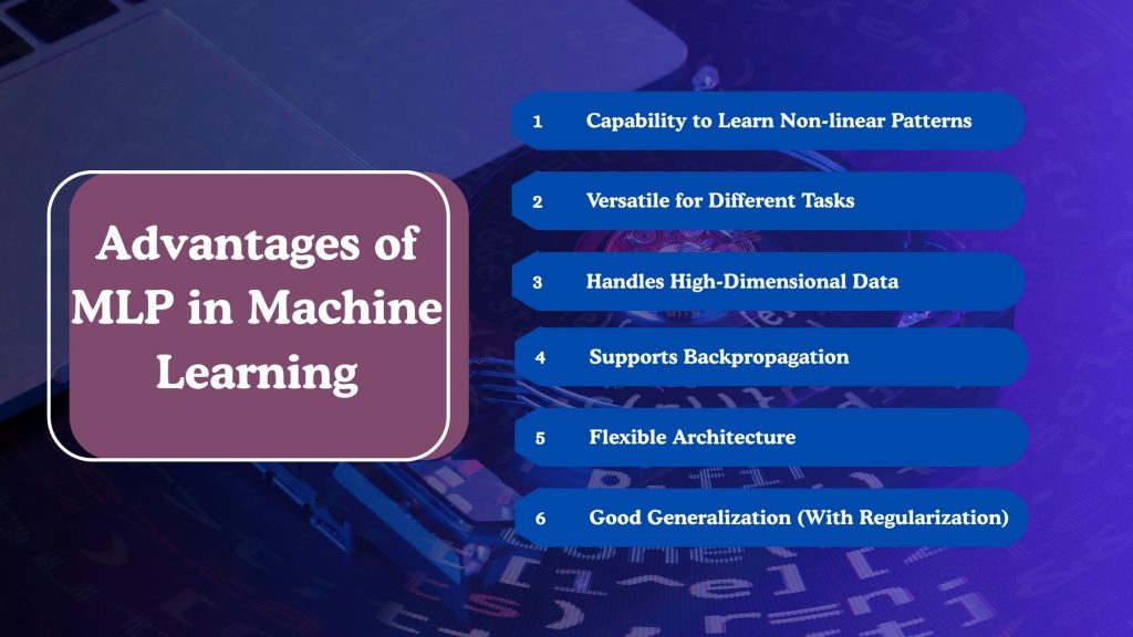
Capability to Learn Non-linear Patterns
One of the most important strengths of an MLP is its ability to learn complex, non-linear relationships between input and output variables. Traditional linear models fall short in such scenarios, whereas MLPs, equipped with multiple hidden layers and non-linear activation functions, can effectively model these intricate patterns.
📌 Use Case: In fraud detection systems, non-linear patterns in transaction data are often key indicators. MLPs excel in identifying such anomalies.
Versatile for Different Tasks
Whether you’re dealing with classification, regression, or even multi-label prediction, MLPs can be adapted to fit various problems. Their architecture is flexible enough to accommodate different types of outputs based on the task requirements.
✅ Can be used for:
- Image classification
- Time series prediction
- Text sentiment analysis
- Customer churn modeling
🔗 Explore More: Learn how businesses apply MLPs and similar models in our Data Science in Marketing blog.
Handles High-Dimensional Data
MLPs perform well even when the input feature space is large—a common challenge in real-world scenarios such as genetics, text mining, and e-commerce recommendation systems. With enough hidden units and regularization, they can extract meaningful patterns without overfitting.
Supports Backpropagation
A major advantage of MLPs is that they utilize backpropagation, a supervised learning technique that efficiently updates the network’s weights to minimize prediction errors. This algorithm allows MLPs to scale and learn from data in a structured way, making training feasible for large datasets.
Flexible Architecture
MLPs can have any number of hidden layers and neurons per layer, providing developers with the flexibility to design architectures tailored to complexity, data type, and performance requirements. This tunability enables optimization in terms of speed, accuracy, and generalization.
🛠️ Tip: While deeper networks can capture more complex patterns, they may also be prone to overfitting if not regularized properly.
Good Generalization (with Regularization)
When trained with proper techniques, such as dropout, L2 regularization, and early stopping, MLPs can generalize well to unseen data. This is particularly essential in real-world applications where test environments differ significantly from the training data conditions.
💬 Example: In email spam detection, an MLP can continue to classify new types of spam messages accurately, even if the exact pattern wasn’t seen during training.
These advantages make the Multilayer Perceptron in ML a go-to model for a broad range of predictive tasks. However, despite their strengths, MLPs also come with some challenges.
Limitations of MLP in Machine Learning
While the Multilayer Perceptron is a foundational model in many AI systems, it isn’t without drawbacks. Despite its flexibility and wide applicability, several limitations render it less than ideal for certain tasks, particularly when dealing with scalability, computational constraints, or limited data availability.
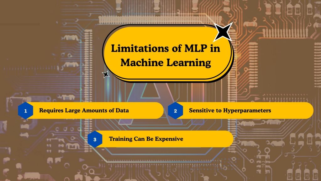
Requires Large Amounts of Data
One of the key limitations of an MLP in Machine Learning is its dependency on large volumes of labeled data. Since MLPs are supervised learning models, they need many input-output examples to learn patterns effectively.
If the dataset is too small, the model may not be able to capture underlying relationships and can end up overfitting, meaning it memorizes the training data rather than generalizing from it. In domains such as healthcare or finance, where collecting labeled data is costly or time-consuming, this dependency poses a significant challenge.
Sensitive to Hyperparameters
Another significant drawback lies in the MLP’s sensitivity to hyperparameters. Choosing the right learning rate, number of hidden layers, number of neurons per layer, activation functions, and optimization algorithms can greatly influence model performance.
Poorly selected hyperparameters can lead to inefficient training, slow convergence, or complete failure to learn. Often, practitioners have to invest considerable time in fine-tuning these parameters through trial and error, which delays development and increases computational overhead.
Training Can Be Computationally Expensive
Training an MLP, especially one with deep architecture, can be computationally demanding. As the number of layers and neurons increases, the volume of computations grows exponentially. Each iteration during training involves calculating gradients, updating weights, and propagating errors back through the network.
Without high-performance computing resources such as GPUs or cloud-based accelerators, training times can become excessively long. This makes MLPs less feasible for teams operating under tight budgets or deadlines, especially when rapid experimentation is required.
Want to Build High-Performance Models Using MLPs?
Discover how Multilayer Perceptrons enhance prediction accuracy and adapt to diverse business challenges.
How MLP in Machine Learning Works: Step-by-Step Process
To truly understand the capabilities of a Multilayer Perceptron, it’s essential to examine how it operates during both the training and prediction phases. From feeding in raw data to making accurate predictions, every stage in an MLP in Machine Learning is carefully designed to optimize learning and performance.
Below is a detailed breakdown of the process, along with code insights that illustrate how it works in practice.
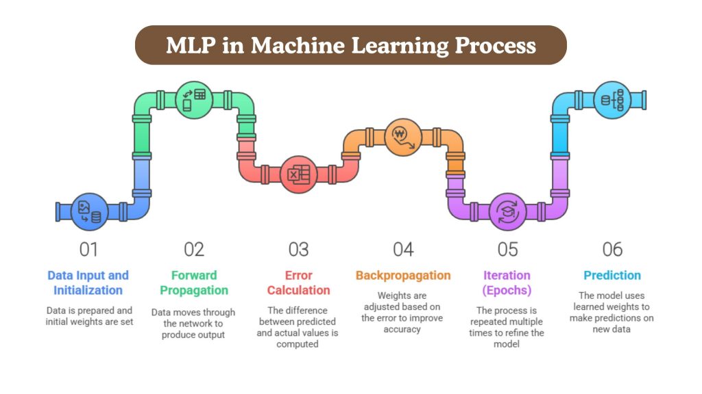
Data Input and Initialization
The journey begins with feeding structured input data into the network. Each input feature corresponds to a neuron in the input layer. Before training starts, weights and biases are initialized—either randomly or using optimized methods, such as Xavier initialization. This setup impacts the initial direction of learning.
Here’s how input and weight initialization typically look using TensorFlow/Keras:
python
from tensorflow.keras.models import Sequential
from tensorflow.keras.layers import Dense
# Define an MLP with 10 input features
model = Sequential()
model.add(Dense(64, activation='relu', input_shape=(10,)))
💡 Tip: Always normalize input data (e.g., using MinMaxScaler or StandardScaler) to speed up learning and improve convergence.
Forward Propagation
In this stage, data passes through the network from input to output. Each neuron calculates a weighted sum of inputs, adds a bias, and applies an activation function like ReLU or Sigmoid to determine its output.
Mathematically, this can be represented as:
z=∑(w⋅x)+b,a=activation(z)z = \sum (w \cdot x) + b,\quad a = \text{activation}(z)z=∑(w⋅x)+b,a=activation(z)
In code, forward propagation is typically handled automatically by libraries like Keras. The line below adds another hidden layer with 32 neurons and ReLU activation:
python
model.add(Dense(32, activation='relu'))
💡 Tip: Using ReLU in hidden layers and Sigmoid or Softmax in output layers is a common and effective combination.
Error Calculation
Once the prediction is made, the model compares it to the actual label using a loss function. This error (or loss) indicates to the model how far it is from the correct solution.
For binary classification, the loss function might be binary cross-entropy:
python
model.compile(optimizer='adam', loss='binary_crossentropy', metrics=['accuracy'])
💡 Example: If the model predicts 0.9 and the actual label is 1, the loss will be small. But if the model predicts 0.1, the loss will be large, motivating a bigger weight update.
Backpropagation
Backpropagation is the core of learning. It calculates the gradient of the loss with respect to each weight in the network. These gradients instruct the model on how to adjust its weights to minimize error.
The optimizer updates the weights using these gradients. In Keras, this happens during training and doesn’t require manual implementation.
🔍 Behind the Scenes: TensorFlow handles this with automatic differentiation and optimizers like Adam, SGD, or RMSprop.
Iteration (Epochs)
Training is an iterative process, repeating forward and backward passes over several epochs. One epoch = one complete pass through the training dataset.
python
model.fit(X_train, y_train, epochs=50, batch_size=32, validation_split=0.2)
The model improves its performance over epochs by minimizing the loss. Early stopping techniques are often used to prevent overfitting.
💡 Tip: Always monitor validation loss. If it starts increasing while training loss decreases, the model might be overfitting.
Prediction
After training, the model is ready to make predictions on new data. Forward propagation is run once more, but without updating any weights.
python
predictions = model.predict(X_test)
These outputs can then be interpreted as class labels or probabilities, depending on the problem.
🎯 Example: In a spam email classifier, the model may output 0.95 for spam and 0.05 for non-spam. You can set a threshold (e.g., 0.5) to classify the message.
This step-by-step process illustrates how an MLP in Machine Learning goes from raw input to intelligent output, learning through repeated exposure to data and feedback. With just a few lines of code and a good dataset, you can begin training powerful predictive models for real-world tasks.
How Can BigDataCentric Help You Learn Machine Learning Concepts?
Mastering machine learning can seem overwhelming, especially with complex architectures like Multilayer Perceptrons, evolving frameworks, and a rapidly changing technological landscape. That’s where BigDataCentric steps in to simplify your learning and development journey. Whether you’re a beginner aiming to grasp foundational concepts or a business professional looking to apply machine learning models practically, we offer tailored support at every level.
At BigDataCentric, we specialize in designing and deploying real-world machine learning and deep learning architectures, including MLPs, for diverse domains like healthcare, finance, retail, and manufacturing. Our team of experts can help you build, train, and optimize models that solve complex problems — all while keeping scalability and performance in mind. We not only offer end-to-end machine learning development services but also focus on education through real implementation, so you can learn by doing.
Additionally, our Custom Machine Learning Development Services are ideal for organizations aiming to integrate AI-driven solutions without relying solely on pre-packaged tools. We guide you through data preparation, model selection (like choosing between MLPs, CNNs, or transformers), and even assist in post-deployment monitoring and improvement.
Suppose you’re curious about how MLPs can support business growth. In that case, we’ve covered real-world use cases in areas like Data Science in Banking, AI in Energy Management, and Predictive Marketing — demonstrating how machine learning is transforming traditional industries.
Whether you’re looking to explore MLPs further or want to design an end-to-end ML pipeline, BigDataCentric offers the resources, expertise, and support to turn concepts into intelligent solutions.
Need Expert Help with MLP Implementation?
Let BigDataCentric guide you through building powerful Multilayer Perceptron models tailored to your business goals — from concept to deployment.
In Bottom Line
The MLP in Machine Learning continues to play a vital role in building predictive models that can handle everything from structured business data to complex, non-linear relationships. While more specialized neural networks, such as CNNs or LSTMs, dominate certain fields, the Multilayer Perceptron remains an essential architecture, especially for those starting or working on classification and regression tasks across diverse domains.
Its simplicity, adaptability, and ability to scale make it a powerful tool in the modern machine learning toolbox. However, like any technology, it comes with limitations, requiring careful data preparation, tuning, and computational resources to unlock its full potential.
Whether you’re experimenting with your first neural network or implementing MLPs as part of larger deep learning architectures, understanding how they work — from initialization to prediction — equips you to make smarter decisions in your machine learning journey. And with the right partner, like BigDataCentric, these models can be transformed into real-world solutions that drive measurable business impact.
FAQs
-
What is the difference between perceptron and multi-layer perceptron?
A perceptron is a single-layer neural network used for binary classification. In contrast, a multi-layer perceptron (MLP) has one or more hidden layers, allowing it to model complex, non-linear relationships and solve more advanced tasks.
-
Can MLP be used for regression tasks?
Yes, MLPs can be used for regression tasks by adjusting the output layer (typically using a linear activation) and selecting an appropriate loss function like Mean Squared Error (MSE).
-
Can MLPs be used for image or text tasks?
MLPs can be applied to image or text data, but they are not ideal due to their inability to capture spatial (like CNNs) or sequential (like RNNs) structures efficiently. Preprocessing is often required.
-
What Are Common Activation Functions Used in Mlps and Why?
Common activation functions include ReLU (fast and avoids vanishing gradients), Sigmoid (for probability outputs), and Tanh (centered at zero). They introduce non-linearity, enabling the network to learn complex patterns.
-
How do MLPs differ from other neural network architectures like CNNs and RNNs?
MLPs are fully connected and process fixed-size input. CNNs are designed for spatial data (images), capturing local features, while RNNs handle sequential data (text/time series) by maintaining temporal context.

About Author
Jayanti Katariya is the CEO of BigDataCentric, a leading provider of AI, machine learning, data science, and business intelligence solutions. With 18+ years of industry experience, he has been at the forefront of helping businesses unlock growth through data-driven insights. Passionate about developing creative technology solutions from a young age, he pursued an engineering degree to further this interest. Under his leadership, BigDataCentric delivers tailored AI and analytics solutions to optimize business processes. His expertise drives innovation in data science, enabling organizations to make smarter, data-backed decisions.


